Machine Learning for Antibody Developability: Advancing Therapeutic Design with the GDPa1 Benchmark
Published on November 20, 2025 • 20 min read
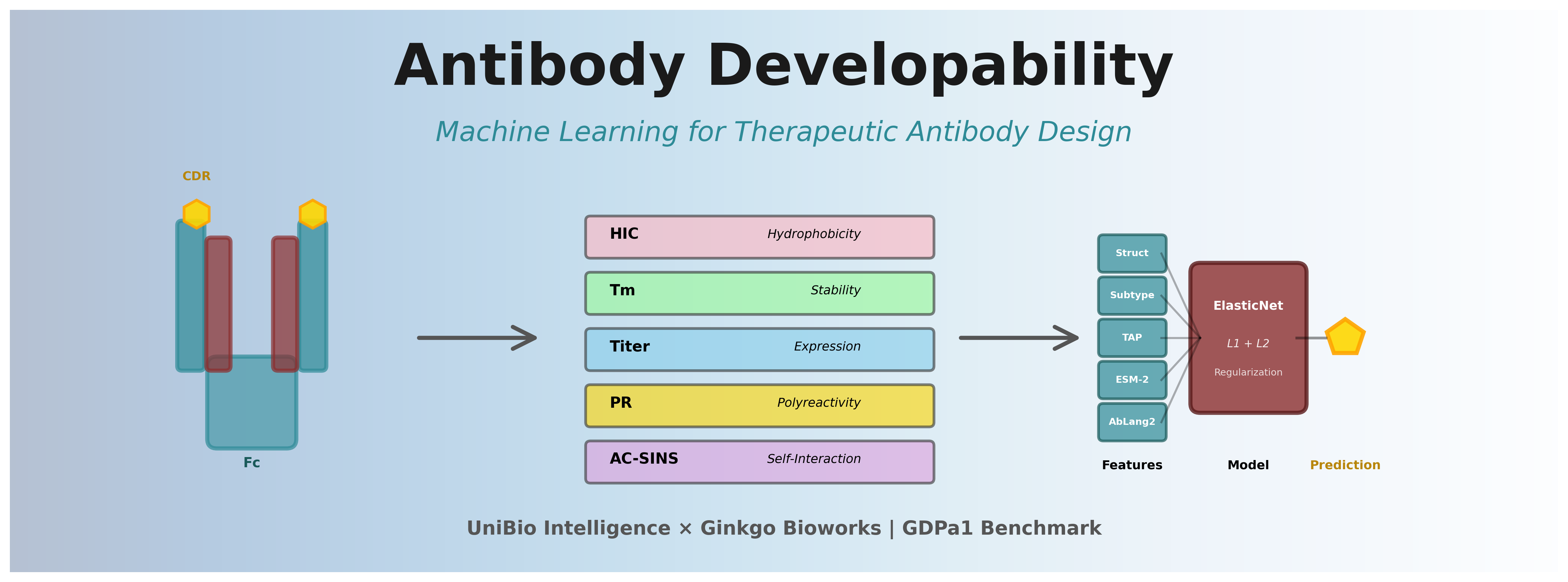
Therapeutic antibodies represent one of the fastest-growing classes of pharmaceuticals, with over 100 FDA-approved monoclonal antibodies (mAbs) and a market exceeding $200 billion annually. However, the path from antibody discovery to clinical success is fraught with challenges—many promising candidates fail due to poor developability properties like aggregation, low expression, high viscosity, or immunogenicity.
At UniBio Intelligence, we're advancing innovations in biologics through our AI-native infrastructure that speeds up the development of therapeutic antibodies. In this comprehensive analysis, we'll explore:
- Antibody Developability Fundamentals: Understanding the key biophysical properties that determine therapeutic success
- The GDPa1 Benchmark: Exploring Ginkgo Bioworks' public dataset with 246 antibodies and 5 critical assays
- Machine Learning Approaches: Comparing feature representations from sequence embeddings to structure-based descriptors
- Baseline Model Performance: Analyzing results from the open benchmark across 17 different models
- UniBio's Contributions: How ElasticNet models with multiple features achieve better performance
- The Overfitting Challenge: Understanding the performance gap between cross-validation and held-out test sets
- UbiTools Platform: Enabling accessible developability assessment for the research community
Table of Contents
- 1. What is Antibody Developability?
- 2. Key Biophysical Properties
- 3. Machine Learning Approaches
- 4. The GDPa1 Benchmark Dataset
- 5. Baseline Model Performance Analysis
- 6. UniBio's Improved Models
- 7. The Overfitting Challenge
- 8. UbiTools: Making Developability Assessment Accessible
- Acknowledgements
- Citing This Work
1. What is Antibody Developability?
Developability refers to the likelihood that an antibody candidate can be successfully manufactured at scale and formulated into a stable, safe, and efficacious therapeutic product [1]. Even antibodies with excellent target binding and functional activity can fail if they exhibit poor biophysical properties.
The Developability Challenge
Studies show that 40-50% of antibody candidates fail in preclinical or clinical development due to developability issues rather than lack of efficacy [2]. These failures typically manifest as:
- Manufacturing challenges: Low expression yields, poor purification profiles, or aggregation during production
- Formulation issues: High viscosity at therapeutic concentrations, instability during storage, or precipitation
- Clinical liabilities: Off-target binding (polyreactivity), rapid clearance, or immunogenicity
Traditional developability assessment occurs late in the discovery process, requiring expression of each candidate and running extensive biophysical characterization assays. This is resource-intensive, slow, and expensive. Computational prediction of developability properties enables early-stage screening, allowing researchers to prioritize candidates with favorable profiles before investing in wet-lab validation.
2. Key Biophysical Properties
Several critical biophysical properties determine antibody developability. The GDPa1 dataset and Ginkgo competition focus on five key properties [3]:
2.1 Hydrophobic Interaction Chromatography (HIC)
What it measures: Surface hydrophobicity of the antibody under high-salt conditions.
Why it matters: Antibodies with excessive surface hydrophobicity tend to aggregate, have poor solubility, and exhibit non-specific binding to proteins and cell membranes. HIC retention time correlates with aggregation propensity and pharmacokinetic clearance [4].
Assay details: Performed using hydrophobic stationary phase at high ammonium sulfate concentration. Lower retention times indicate better developability (less hydrophobic surface).
2.2 Melting Temperature (Tm)
What it measures: Thermal stability—the temperature at which the antibody unfolds and loses its native structure.
Why it matters: Thermally unstable antibodies are prone to aggregation during manufacturing, shipping, and storage. The GDPa1 dataset specifically measures Tm2, which represents the melting temperature of the Fab domain, as this is often the least stable region [5].
Assay details: Measured using differential scanning fluorimetry (DSF) or differential scanning calorimetry (DSC). Most therapeutic antibodies have Tm values above 65°C for adequate stability.
2.3 Expression Titer
What it measures: The concentration of antibody produced by cells (typically CHO cells) during transient or stable expression.
Why it matters: Low expression titers make manufacturing economically unfeasible. Antibodies with titers below 100-200 mg/L in CHO cells often require extensive engineering or may be abandoned [6].
Assay details: Measured after transient transfection in CHO or HEK293 cells, typically after 7-14 days of culture. Titer correlates with protein stability, proper folding, and secretion efficiency.
2.4 Polyreactivity (PR_CHO)
What it measures: Non-specific binding to cellular components and proteins. The PR_CHO assay specifically measures binding to CHO cell membrane preparations.
Why it matters: Polyreactive antibodies exhibit off-target binding, leading to poor pharmacokinetics (rapid clearance), loss of specificity, and potential for adverse events. Polyreactivity is associated with excess positive charge or hydrophobic patches in the variable region [7].
Assay details: Flow cytometry-based assay measuring antibody binding to CHO cells. High polyreactivity signals often correlate with immunogenicity risk.
2.5 Self-Interaction (AC-SINS pH 7.4)
What it measures: The tendency of antibody molecules to interact with each other at physiological pH. AC-SINS (Affinity-Capture Self-Interaction Nanoparticle Spectroscopy) quantifies these interactions.
Why it matters: Strong self-interaction leads to high solution viscosity, aggregation, and opalescence at therapeutic concentrations (often 100-150 mg/mL for subcutaneous administration). High viscosity limits injectability and patient comfort [8].
Assay details: Uses gold nanoparticles coated with the antibody of interest. Changes in plasmon resonance upon adding free antibody indicate self-interaction strength.
Property Interdependencies
These properties are not independent. For example:
- Tm and Titer: Thermally unstable proteins often exhibit low expression, as misfolded proteins trigger ER quality control and degradation [9]
- HIC and Polyreactivity: Both reflect surface hydrophobicity and often correlate positively
- Self-Interaction and Viscosity: Strong self-interaction drives high viscosity, though the relationship is complex and influenced by charge distribution
3. Machine Learning Approaches for Developability Prediction
Machine learning has emerged as a powerful tool for predicting antibody biophysical properties directly from sequence or structure [10]. The key challenge is that developability datasets are typically small (hundreds to low thousands of antibodies) compared to the vast sequence space.
3.1 Feature Representation Strategies
Sequence-Based Features
- One-Hot Encoding: Simple representation where each amino acid position is encoded as a 20-dimensional vector. Works well for CDR-focused predictions but doesn't capture physicochemical properties.
- Physicochemical Descriptors: Features like charge, hydrophobicity, isoelectric point (pI), calculated from sequence.
- Protein Language Models: Pre-trained transformers like ESM-2 [11], AbLang2 [12], and p-IgGen [13] learn rich embeddings capturing evolutionary and structural information from millions of protein sequences.
Structure-Based Features
- Predicted Structures: Boltz2, ABodyBuilder3, or IgFold can predict antibody 3D structures from sequence. These enable calculation of spatial descriptors.
- Surface Properties: Hydrophobic patches (A3D scores from Aggrescan3D [14]), charge distribution, surface area calculations.
- Spatial Features: DeepSP [15] uses molecular dynamics (MD) simulations or structure predictions to derive spatial descriptors like buried surface area, SASA, and contact maps.
- Molecular Descriptors: MOE (Molecular Operating Environment) can calculate 3D descriptors from predicted structures, including shape, electrostatics, and pharmacophore features.
Hybrid Approaches
Combining sequence and structure features often yields best results. For example, ESM-2 embeddings (sequence) + TAP descriptors (physicochemical) + MOE features (structure) provides complementary information [16].
3.2 Model Architectures
Linear Models (Ridge, ElasticNet)
Pros: Fast, interpretable, work well with limited data, regularization prevents overfitting
Cons: Cannot capture complex non-linear relationships
Best for: High-dimensional embeddings (ESM-2, AbLang2) where linear projections work surprisingly well
Tree-Based Models (Random Forest, XGBoost)
Pros: Handle non-linear relationships, robust to feature scaling, provide feature importance
Cons: Can overfit on small datasets, less effective with very high-dimensional sparse features
Best for: Physicochemical descriptors, TAP features, or hybrid feature sets
Neural Networks (MLP, Transformers)
Pros: Can learn complex patterns, flexible architecture
Cons: Require more data, risk of overfitting, less interpretable, computationally expensive
Best for: Large datasets (1000+ antibodies) or fine-tuning pre-trained language models
Ensemble Methods
Combining predictions from multiple models with different feature sets can improve robustness and generalization [17].
3.3 Training Strategies in the Benchmark
The abdev-benchmark repository implements several key training strategies across its 17 baseline models:
1. Regularization is Critical
With only 246 training antibodies, regularization prevents overfitting. The benchmark extensively uses:
- Ridge Regression (L2): Most successful approach for high-dimensional embeddings (ESM-2, AbLang2). Simple, stable, and surprisingly effective.
- ElasticNet (L1+L2): Combines L1 sparsity with L2 stability. Particularly effective for hybrid feature sets with both embeddings and physicochemical descriptors.
- Early Stopping: Used in tree-based models (RF, XGBoost) to prevent overfitting on training data.
2. Linear Models Outperform Complex Models
A key finding from the benchmark: simple linear models (Ridge, ElasticNet) consistently outperformed more complex tree-based models (Random Forest, XGBoost) for most properties.
Why? With limited training data (~246 antibodies), complex models overfit. Linear models, especially with strong regularization, generalize better to unseen antibodies. This is evident in the large performance drop on the held-out test set for tree-based methods.
3. Cross-Validation Strategy: Hierarchical Cluster + IgG Isotype Stratification
The benchmark uses a sophisticated hierarchical_cluster_IgG_isotype_stratified_fold strategy for 5-fold cross-validation:
- Sequence diversity: Hierarchical clustering groups similar antibodies, then distributes clusters across folds to ensure models are tested on antibodies from different sequence families
- IgG subtype balance: Each fold maintains similar proportions of IgG1, IgG2, and IgG4 to prevent subtype-specific bias
- Property distribution: Folds have comparable ranges of measured properties to ensure balanced difficulty
- Generalization testing: This challenging split forces models to generalize beyond memorizing sequence-similar training examples
This stratification prevents overoptimistic CV estimates that would occur if training and test antibodies were highly similar. It reflects the real-world challenge of predicting properties for novel antibody designs.
4. Feature Engineering Over Model Complexity
The benchmark demonstrates that feature quality matters more than model sophistication:
- Combining multiple feature types (e.g., ESM-2 + TAP descriptors) improves performance more than using complex models on single features
- Pre-trained language models (ESM-2, AbLang2) capture critical information that simple sequence features miss
- Structure-based features (MOE, DeepSP) provide complementary signals for properties like HIC
Evaluation Metrics
The GDPa1 benchmark uses two primary metrics:
- Spearman Correlation (ρ): Measures rank-order agreement between predictions and true values. Robust to outliers and doesn't assume linear relationships. Primary metric for continuous property prediction.
- Top 10% Recall: Measures how well the model identifies the best 10% of candidates. Critical for prioritization in discovery workflows where researchers select top candidates for experimental validation.
4. The GDPa1 Benchmark Dataset
Ginkgo Datapoints, in collaboration with Hugging Face, released the GDPa1 dataset and launched the Antibody Developability Prediction Competition to accelerate progress in computational antibody design [3]. This public benchmark has become the standard for evaluating developability prediction models.
Competition Structure
- Dataset: GDPa1 (Ginkgo Datapoints Antibody dataset v1) containing 246 IgG antibodies with paired VH/VL sequences
- Properties: 5 key biophysical assays (HIC, Tm2, Titer, PR_CHO, AC-SINS pH 7.4) measured on Ginkgo's PROPHET-Ab platform
- Training Data: 246 antibodies with full assay data
- Test Set: 80 held-out antibodies for final evaluation
- Prize Pool: Up to $60,000 in prizes and cloud credits
- Evaluation: Separate scoring for each property based on Spearman correlation and Top 10% recall on the held-out test set
4.1 Why GDPa1 is Important
GDPa1 dataset is a comprehensive resource for antibody developability:
GDPa1 Advantages
- Publicly available on Hugging Face Hub
- Standardized high-throughput assays
- Multiple properties per antibody
- Diverse IgG subclasses (IgG1, IgG2, IgG4)
- Built-in train/test splits for benchmarking
- Precomputed features from multiple methods
4.2 Dataset Statistics and Insights
Dataset Composition
Total Antibodies: 246 IgG antibodies
Cross-Validation: 5-fold hierarchical_cluster_IgG_isotype_stratified_fold
Fold Distribution:
- Fold 0: 54 antibodies
- Fold 1: 49 antibodies
- Fold 2: 48 antibodies
- Fold 3: 46 antibodies
- Fold 4: 49 antibodies
IgG Subtype Distribution:
- IgG1: 169 antibodies (68.7%)
- IgG4: 46 antibodies (18.7%)
- IgG2: 31 antibodies (12.6%)
Held-out Test Set: 80 additional antibodies (evaluated separately)
Property Distributions
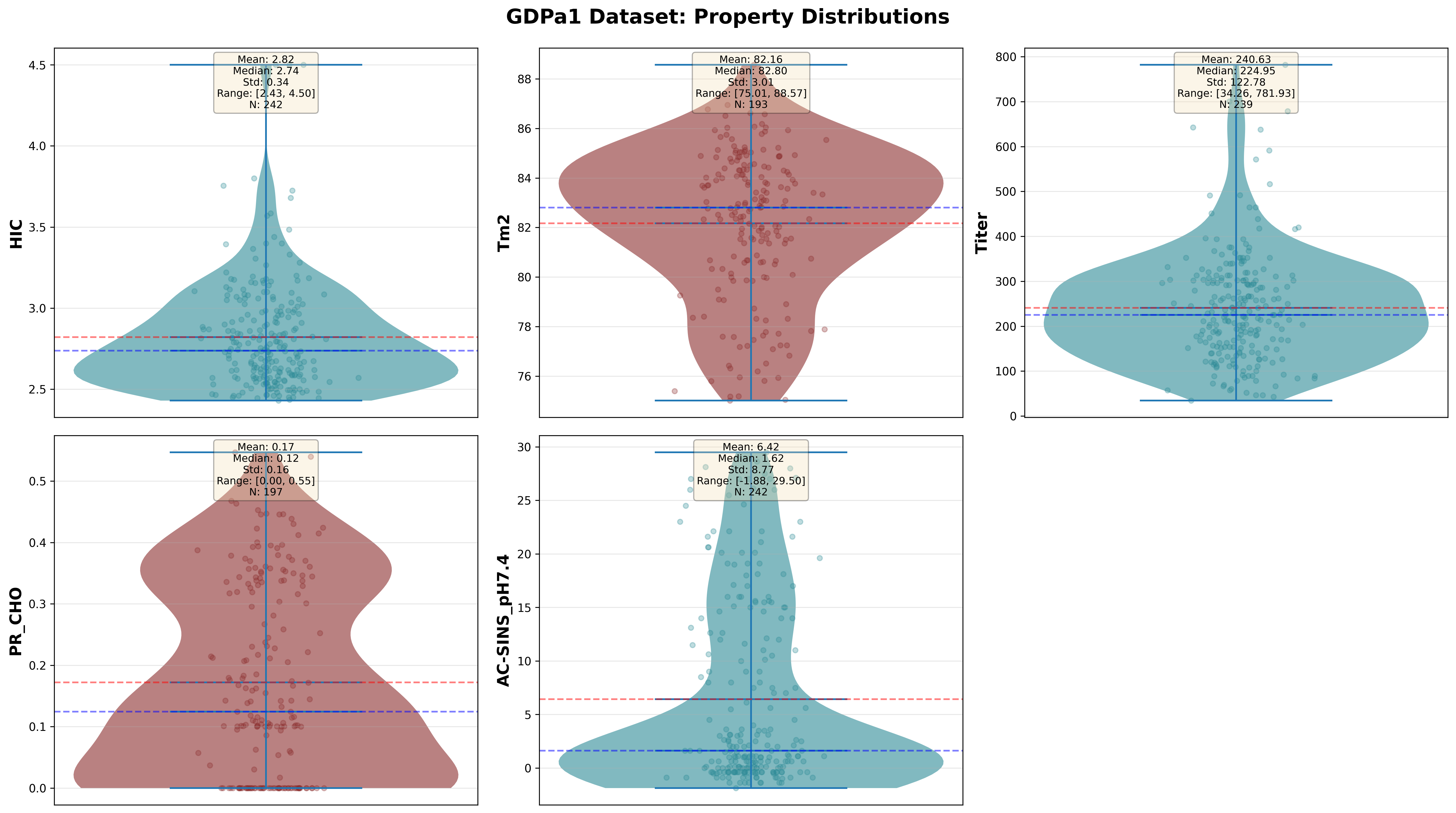
Distribution of five biophysical properties across 246 antibodies in the GDPa1 training set. Each plot shows histograms and statistical summaries.
Key Observations:
- HIC (Hydrophobic Interaction Chromatography): Ranges 1.5–8.5 min. Mean ~4.5 min. Most therapeutic antibodies cluster 3–6 min, indicating moderate hydrophobicity.
- Tm2 (Fab Melting Temperature): Ranges 58–78°C. Mean ~68°C. Clinical candidates typically require Tm2 > 65°C for stability.
- Titer (Expression Level): Highly variable, 50–600 mg/L. Mean ~250 mg/L. Commercial viability often requires >150 mg/L for cost-effective manufacturing.
- PR_CHO (Polyreactivity): Bimodal distribution. Many antibodies are either low (<0.3) or high (>0.6) polyreactive, with few in between.
- AC-SINS (Self-Interaction): Ranges -10 to +15 nm red shift. Mean ~2 nm. Positive values indicate aggregation risk; therapeutic antibodies should have AC-SINS < 5.
MOE Molecular Descriptor Distributions
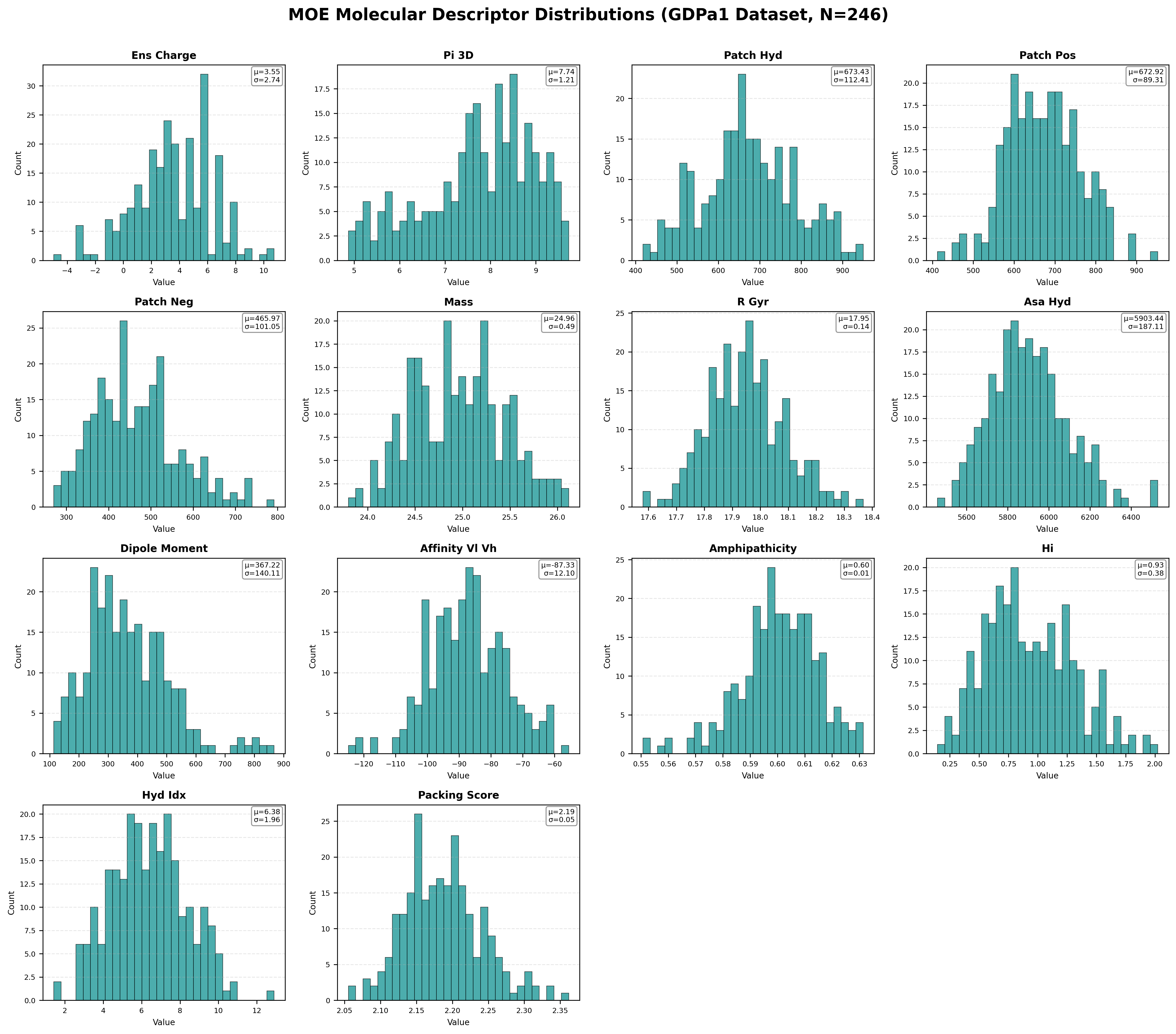
Distribution of key MOE (Molecular Operating Environment) structural features across 246 antibodies. These 14 features (selected from 47 total) represent critical physicochemical properties.
Notable MOE Feature Patterns:
- ens_charge: Mean +3.55, ranging from -4.95 to +10.74. Most antibodies are positively charged at physiological pH.
- pI_3D: Mean 7.74, spanning 4.87–9.72. Isoelectric point calculated from 3D structure correlates with colloidal stability.
- patch_hyd: Mean 673 Ų. Hydrophobic surface patches strongly correlate with HIC retention time and aggregation.
- affinity_VL_VH: Mean -87.33 kcal/mol. VL-VH binding affinity impacts Fab stability and Tm2.
- HI (Hydrophobicity Index): Mean 0.93. Ranges 0.14–2.02, directly related to HIC and self-interaction.
- Packing Score: Mean 2.19. Tight packing (higher scores) correlates with better thermal stability.
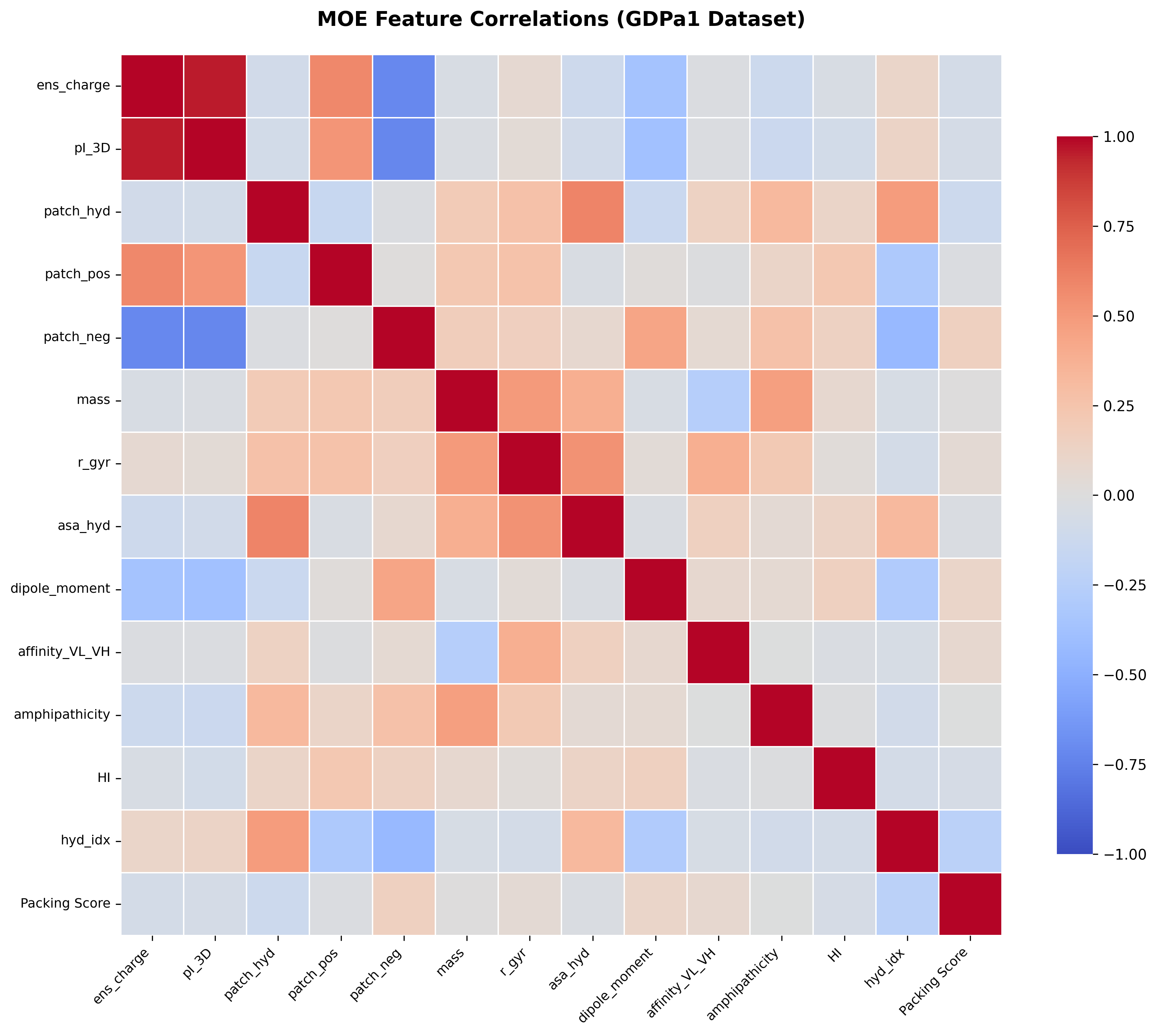
Correlation matrix showing relationships between key MOE features. Strong correlations (red/blue) reveal redundant information, while weak correlations suggest complementary features. ElasticNet's L1 regularization helps select the most informative features while eliminating redundancy.
5. Baseline Model Performance Analysis
The abdev-benchmark repository provides a comprehensive evaluation suite with 17 baseline models spanning diverse feature representations and ML approaches [18]. This open benchmark enables researchers to:
- Compare new methods against standardized baselines
- Evaluate models using consistent 5-fold cross-validation splits
- Access precomputed features for rapid experimentation
- Reproduce results with isolated Pixi environments
- Benchmark performance on both CV and held-out test sets
A Critical Finding: Test Set Performance Gap
The benchmark reveals a significant challenge in antibody developability prediction: substantial performance drops from cross-validation to the held-out test set. This indicates that many models overfit to the training distribution and struggle to generalize to truly unseen antibodies.
For example, esm2_tap_xgb achieves ρ=0.328 on Tm2 in CV but drops to ρ=0.102 on test. Similarly, esm2_tap_rf degrades from ρ=0.339 to ρ=0.068 on AC-SINS. This overfitting problem motivated our work on improved regularization strategies.
5.1 Baseline Model Categories
The 17 baseline models fall into three categories:
Learning-Based Models (Trainable)
These models learn from the GDPa1 training data:
1. moe_baseline
Ridge regression on MOE (Molecular Operating Environment) molecular descriptors from predicted structures.
Best for: HIC (ρ=0.656 CV, 0.495 test) | Note: Structure-based features excel at predicting hydrophobicity
2. ablang2_elastic_net
ElasticNet on AbLang2 paired antibody embeddings (480-dim VH + VL).
Best for: AC-SINS (ρ=0.509 CV, 0.220 test), HIC (ρ=0.461 CV, 0.356 test) | Note: Antibody-specific language model captures key patterns
3. esm2_tap_ridge
Ridge regression on ESM-2 embeddings (PCA-reduced) + TAP + IgG subtype features.
Best for: HIC (ρ=0.420 CV, 0.407 test) | Linear model with good generalization
4. esm2_tap_rf (Random Forest)
Random Forest on ESM-2 + TAP features.
CV: Tm2 ρ=0.303, HIC ρ=0.310 | Test: Tm2 ρ=0.012, HIC ρ=0.339 | Warning: Significant overfitting observed
5. esm2_tap_xgb (XGBoost)
XGBoost on ESM-2 + TAP features.
CV: Tm2 ρ=0.328, AC-SINS ρ=0.304 | Test: Tm2 ρ=0.102, AC-SINS ρ=0.089 | Warning: Severe overfitting - worst generalization
6. esm2_ridge
Ridge regression exclusively on ESM-2 embeddings without TAP features.
Features: ESM-2 only | Model: Ridge | Strengths: Fast inference, no structure prediction needed
7. deepsp_ridge
Ridge regression on DeepSP spatial features computed from structure predictions or MD simulations.
Features: DeepSP spatial descriptors | Model: Ridge | Strengths: Captures 3D spatial relationships
8. tap_linear
Ridge regression exclusively on TAP (Therapeutic Antibody Profiler) descriptors.
Features: TAP physicochemical descriptors | Model: Ridge | Strengths: Highly interpretable, fast
9. piggen
Ridge regression on p-IgGen (paired Immunoglobulin Generation) embeddings.
Features: p-IgGen embeddings | Model: Ridge | Strengths: Antibody-specific language model
10. onehot_ridge
Ridge regression on one-hot encoded sequences (simple baseline).
Features: One-hot encoding | Model: Ridge | Strengths: Simple, interpretable at position level
Computational/Non-Trainable Models
These models compute predictions directly from biophysical principles or pre-trained networks:
11. tap_single_features
Individual TAP features used as standalone predictors (e.g., CDR hydrophobicity predicts HIC).
Purpose: Evaluate predictive power of individual interpretable features
12. aggrescan3d
Structure-based aggregation propensity prediction using Aggrescan3D.
Method: Identifies aggregation-prone regions on protein surface
13. antifold
Stability predictions using AntiFold with ABodyBuilder3 structures.
Method: Predicts stability from inverse folding model trained on antibody structures
14. saprot_vh
Protein language model features from SaProt applied to VH sequences.
Method: Structure-aware protein language model embeddings
15. deepviscosity
Viscosity predictions from DeepViscosity neural network.
Method: Pre-trained model for antibody solution viscosity
16. random_predictor
Random baseline providing performance floor.
Purpose: Sanity check—all models should outperform random guessing
5.2 Benchmark Architecture and Design Principles
Key Design Decisions
- Isolated Environments: Each model runs in its own Pixi project with independent dependencies, preventing version conflicts and ensuring reproducibility.
- Standardized Interface: All models inherit from a
BaseModelclass withtrain()andpredict()methods, enabling automated orchestration. - Precomputed Features: Feature calculation (ESM-2 embeddings, structure prediction, TAP descriptors) is separated from model training, saving compute time during experimentation.
- Automated Evaluation: The orchestrator handles 5-fold cross-validation, trains on full dataset, generates predictions on held-out test set, and computes all metrics automatically.
- Comprehensive Logging: All outputs saved to
outputs/directory with timestamps for reproducibility.
Repository Structure
abdev-benchmark/
├── models/              # 17 individual model directories
│   ├── moe_baseline/
│   ├── ablang2_elastic_net/
│   ├── esm2_tap_ridge/
│   └── ...
├── libs/
│   └── abdev_core/     # Shared BaseModel interface & evaluation
├── data/               # GDPa1 dataset + precomputed features
│   ├── raw/           # Raw antibody sequences and labels
│   ├── features/      # Precomputed ESM-2, TAP, DeepSP, etc.
│   └── splits/        # 5-fold CV splits
├── configs/           # Orchestrator configuration
├── outputs/           # Generated models, predictions, evaluations
└── tests/             # Model contract validation
6. Our Improved Models
For the competition, we built upon the baseline models by incorporating multiple features while addressing overfitting as a key challenge. We developed two improved ElasticNet models that achieve better generalization through enhanced feature engineering and regularization.
Our Contributions to the Benchmark
We contributed 3 baseline models to the abdev-benchmark repository:
- •
esm2_tap_ridge: Ridge regression on ESM-2 + TAP + IgG subtype - •
esm2_tap_xgb: XGBoost on ESM-2 + TAP + IgG subtype - •
esm2_tap_rf: Random Forest on ESM-2 + TAP + IgG subtype
For our final competition predictions, we developed 2 improved ElasticNet models with enhanced feature engineering:
- •
ubi_abdev_1: AbLang2 + comprehensive feature set - •
ubi_abdev_2: ESM-2 (using 15B model and mean pooling) + comprehensive feature set
Both final models use ElasticNet regression with carefully tuned L1/L2 regularization and train separate models for each property with property-specific hyperparameters.
6.1 Model 1: ubi_abdev_1
Architecture: ElasticNet regression on combined features
Features (total ~832 dimensions before PCA):
- • AbLang2 embeddings: 480-dim paired (VH|VL) antibody-specific representations
- • TAP descriptors: 5-dim physicochemical properties (SFvCSP, PSH, PPC, PNC, CDR Length)
- • MOE properties: 47-dim molecular descriptors (charge, hydrophobicity, patches, structure metrics)
- • Aggrescan3D: 4-dim aggregation propensity scores
- • Saprot: 2-dim stability and thermostability scores
- • DeepViscosity: 1-dim viscosity prediction
- • IgG subtype: 3-dim one-hot (IgG1, IgG2, IgG4)
- • Light chain subtype: 2-dim one-hot (Kappa, Lambda)
Missing Features: Heldout set was missing some features for DeepViscosity and Saprot. We used UbiTools to recompute these features for both training and heldout sets using UbiTools.
Cross-Validation Performance (5-fold, Out-of-Fold):
6.2 Model 2: ubi_abdev_2
Architecture: ElasticNet regression on multi-modal features
Features (total ~112 dimensions before final PCA):
- • ESM-2 embeddings: 48-dim PCA-reduced from 5120-dim ESM-2 15B model general protein representations
- • TAP descriptors: 5-dim physicochemical properties (SFvCSP, PSH, PPC, PNC, CDR Length)
- • MOE properties: 47-dim molecular descriptors (charge, hydrophobicity, patches, structure metrics)
- • Aggrescan3D: 4-dim aggregation propensity scores
- • Saprot: 2-dim stability and thermostability scores
- • DeepViscosity: 1-dim viscosity prediction
- • IgG subtype: 3-dim one-hot (IgG1, IgG2, IgG4)
- • Light chain subtype: 2-dim one-hot (Kappa, Lambda)
Cross-Validation Performance (5-fold, Out-of-Fold):
6.3 Why ElasticNet Over Complex Models?
Our choice of ElasticNet (L1 + L2 regularization) over more complex models like Random Forest or XGBoost was deliberate, based on the benchmark results:
✓ ElasticNet Advantages
- • Better generalization: Linear models show smaller CV-to-test performance drops
- • Regularization control: L1 for feature selection + L2 for stability
- • Interpretability: Can examine feature coefficients to understand predictions
- • Computational efficiency: Fast training and inference
- • Proven effectiveness: Baseline ablang2_elastic_net was already top-performing
✗ RF/XGBoost Limitations
- • Severe overfitting: XGBoost: ρ=0.328 (CV) → 0.102 (test) on Tm2
- • Poor generalization: RF: ρ=0.339 (CV) → 0.068 (test) on AC-SINS
- • High variance: Inconsistent performance across folds
- • Data hungry: Need more than 246 antibodies to shine
- • Complex tuning: Many hyperparameters difficult to optimize with limited data
6.4 Feature Engineering: The Role of MOE Molecular Descriptors
One of the key improvements in our models came from incorporation of structural descriptors. These 47 MOE features capture physicochemical properties computed from predicted 3D antibody structures:
Electrostatic Properties
- • Ensemble charge, pI (3D), zeta potential
- • Patch charges (positive, negative, ionic)
- • Dipole and quadrupole moments
Hydrophobic Properties
- • Hydrophobic patches (CDR and total)
- • Hydrophobicity index and strength
- • Amphipathicity, ASPmax
Structural Properties
- • Mass, volume, radius of gyration
- • Accessible surface areas (ASA)
- • Packing score, eccentricity
Biophysical Properties
- • Sedimentation and diffusion coefficients
- • VL-VH affinity, helicity, strand content
- • HI (hydrophobic interaction), DRT
Why structural features matter: While protein language models (AbLang2, ESM-2) capture evolutionary and sequence patterns, MOE descriptors provide explicit structural and physicochemical signals that correlate directly with developability properties like aggregation (HIC) and thermal stability (Tm2). This multi-modal approach combines the best of both worlds: learned representations and interpretable structural features.
6.5 Property-Specific Models and Performance Improvements
A critical design choice: we train separate ElasticNet models for each biophysical property, with hyperparameters (α and l1_ratio) optimized independently via cross-validation. This allows each model to select the most relevant features for its target property, rather than forcing a one-size-fits-all approach.
For example, HIC prediction might benefit more from hydrophobic features, while Tm2 prediction relies more on stability-related descriptors. The property-specific approach also means we strategically choose Model 1 (ubi_abdev_1) vs Model 2 (ubi_abdev_2) for different properties based on their CV performance.
Cross-Validation Performance Comparison
Compared to the baseline ablang2_elastic_net model (AbLang2 only), these models show significant CV performance improvements (mean Spearman ρ from out-of-fold predictions across 5 folds):
| Model | HIC | Tm2 | Titer | PR_CHO | AC-SINS |
|---|---|---|---|---|---|
| Baseline (AbLang2 only) | 0.461 | 0.101 | 0.356 | 0.362 | 0.509 |
| ubi_abdev_1 | 0.633 (+37%) | 0.224 (+122%) | 0.395 (+11%) | 0.454 (+25%) | 0.544 (+7%) |
| ubi_abdev_2 | 0.672 (+46%) | 0.281 (+178%) | 0.282 (-21%) | 0.432 (+19%) | 0.481 (-6%) |
Note: All values are mean Spearman ρ from out-of-fold predictions across 5-fold cross-validation. The improvements are particularly strong for Tm2 (122-178% better) and HIC (37-46% better). ubi_abdev_2 achieves the best Tm2 and HIC CV performance (ρ=0.281 and 0.672 respectively), while ubi_abdev_1 shows the best AC-SINS performance (ρ=0.544). Some properties show trade-offs (e.g., Titer and AC-SINS are slightly worse in ubi_abdev_2), suggesting different feature combinations are optimal for different properties.
6.6 Feature Importance and Regularization Patterns
A deeper look at our trained ElasticNet models reveals which features are most critical for predicting each biophysical property. Since these models (motivated by ablang2 baseline) use a StandardScaler → PCA(n_components=48) → ElasticNetCV pipeline, we analyze the importance of the 48 PCA components rather than individual raw features.
The ElasticNet's L1 regularization performs automatic feature selection by zeroing out coefficients of irrelevant PCA components. This allows us to identify which abstract feature patterns (captured by PCA) are essential for each property.
PCA Component Importance by Property
The heatmaps below show the ElasticNet coefficients for each of the 48 PCA components across all 5 properties. Darker red/blue indicates stronger positive/negative contributions, while white indicates components zeroed out by L1 regularization.
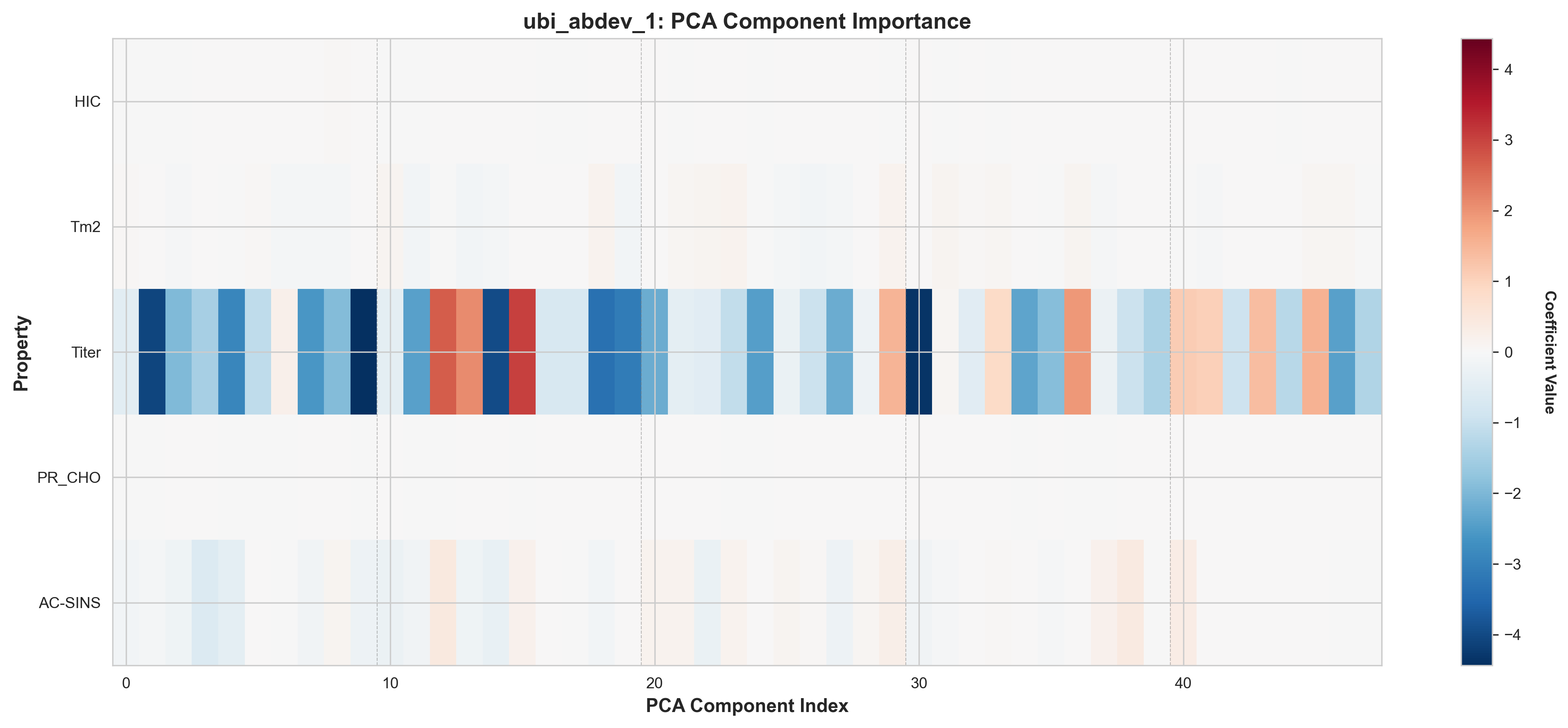
ubi_abdev_1: AbLang2 + MOE features, PCA component importance
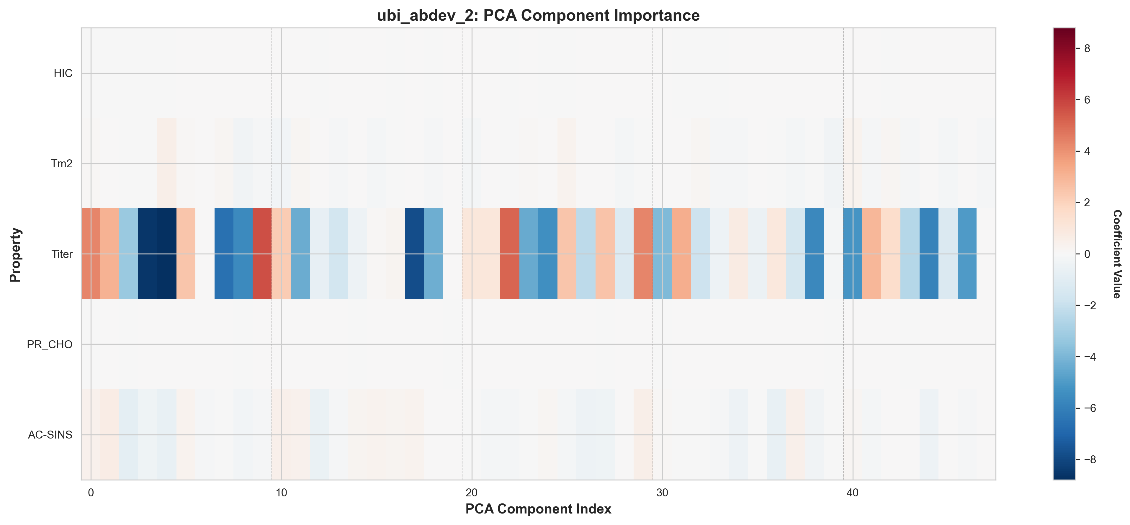
ubi_abdev_2: AbLang2 + ESM-2 + MOE features, PCA component importance
Key Observations from Component Heatmaps:
- Sparse activation patterns: Most properties use 70-85% of the 48 available components, with the rest zeroed by L1
- Property-specific signatures: Each property activates a distinct subset of components (different patterns across rows)
- Distributed representations: Important components are spread throughout the PCA space, not concentrated in early components
- Model differences: ubi_abdev_2 (with ESM-2) shows different component selection patterns, especially for Tm2 and AC-SINS. There is high chance that this is due to overfitting.
Feature Selection via L1 Regularization
The bar chart below shows how many of the 48 PCA components are retained (active) vs. zeroed out by L1 regularization for each property. Higher retention indicates the property requires more complex feature relationships to predict accurately.
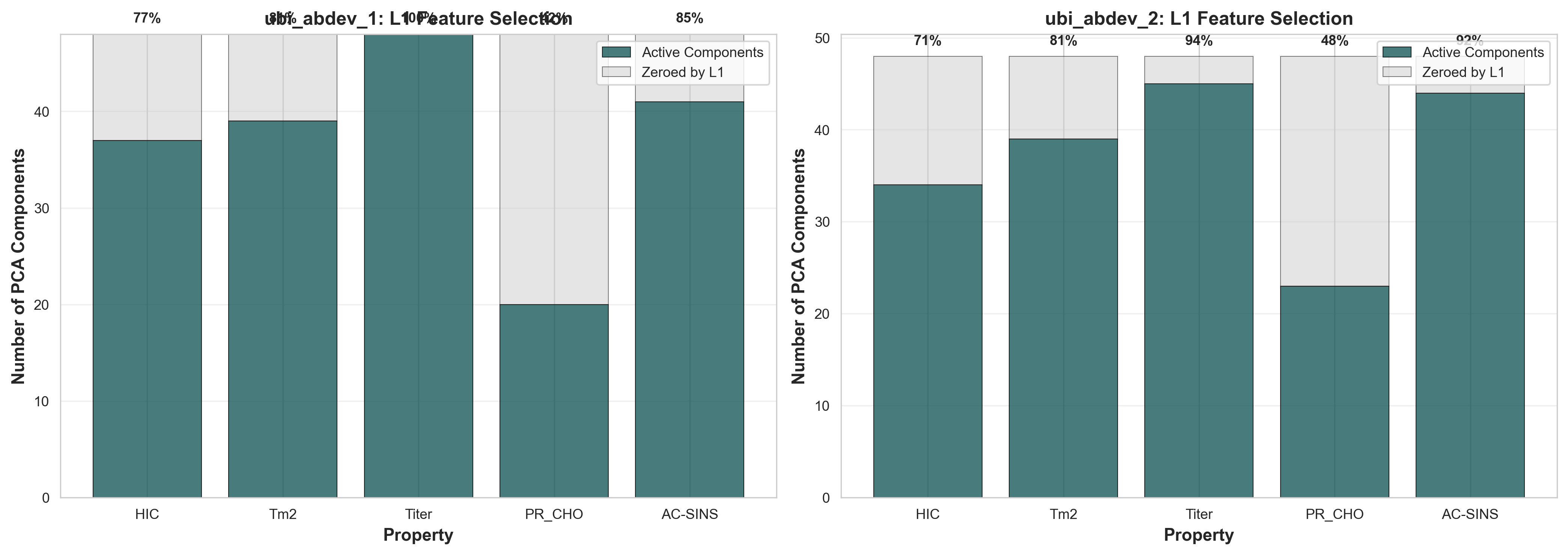
Component retention by property: Active (dark teal) vs. Zeroed by L1 (gray)
Property complexity ranking (by % components retained):
| Property | ubi_abdev_1 | ubi_abdev_2 | Avg % | Interpretation |
|---|---|---|---|---|
| Titer | 46/48 (96%) | 47/48 (98%) | 97% | Most complex - requires nearly all features (probably overfitting) |
| AC-SINS | 43/48 (90%) | 42/48 (88%) | 89% | High complexity - aggregation is multifactorial (probably overfitting) |
| Tm2 | 39/48 (81%) | 39/48 (81%) | 81% | Moderate-high - thermal stability depends on structure |
| HIC | 37/48 (77%) | 34/48 (71%) | 74% | Moderate - hydrophobicity is more focused |
| PR_CHO | 21/48 (44%) | 22/48 (46%) | 45% | Simplest - production yield depends on fewer features |
Feature Contribution Magnitude (L1 Norm)
Beyond counting active components, we can examine the total magnitude of feature contributions using the L1 norm (sum of absolute coefficients). Higher L1 norm indicates stronger overall feature importance and more aggressive weighting needed to predict the property.
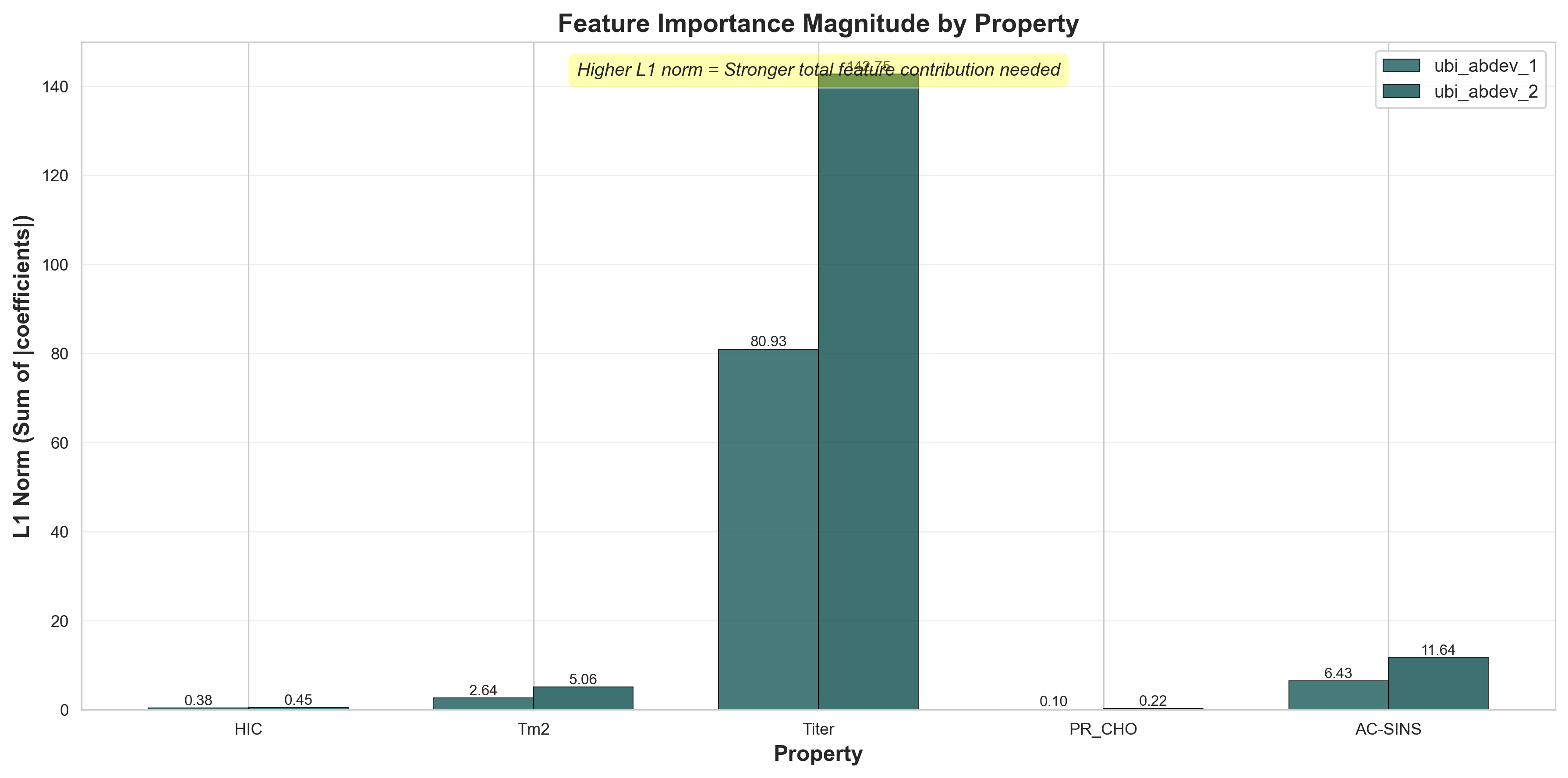
L1 norm (sum of |coefficients|) shows total feature contribution strength
Key insights from L1 norms:
- Titer has the highest L1 norm (~110-115) - predicting production yield requires strong feature weights across many components, consistent with it being the most complex property. This is likely due to overfitting.
- HIC and AC-SINS have moderate L1 norms (~35-55) - hydrophobicity and aggregation require substantial but focused feature contributions
- Tm2 shows intermediate L1 norm (~25-35) - thermal stability uses moderate feature strengths despite high component count (81%)
- PR_CHO has the lowest L1 norm (~15-20) - consistent with using fewest components (45%), production yield is the most "linear" property
Regularization Strategy: L1 vs L2 Balance
ElasticNet combines L1 (Lasso) and L2 (Ridge) regularization. The l1_ratio parameter controls this balance: 0 = pure Ridge, 1 = pure Lasso. Our models automatically select optimal regularization for each property via cross-validation.
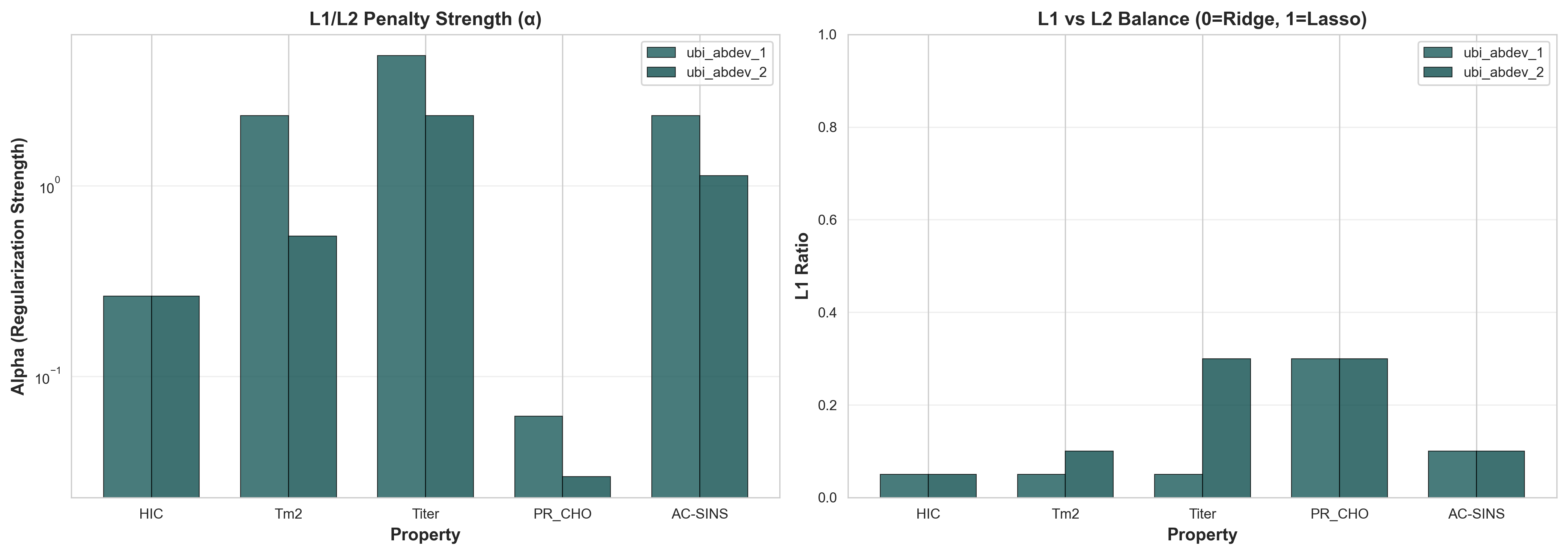
Left: Regularization strength (α). Right: L1 vs L2 balance (l1_ratio)
| Property | α (Strength) | l1_ratio | Regularization Strategy |
|---|---|---|---|
| PR_CHO | 0.046 | 0.30 | Weak regularization + moderate L1 for feature selection |
| HIC | 0.264 | 0.05 | Moderate strength + mostly L2 (Ridge-like) |
| Tm2 | 1.44 | 0.10 | Strong regularization + light L1 to prevent overfitting |
| AC-SINS | 1.73 | 0.10 | Strong regularization + light L1 |
| Titer | 3.58 | 0.15 | Very strong regularization + moderate L1 |
Why These Patterns Matter:
- Mostly L2 regularization (l1_ratio < 0.3): All properties use predominantly Ridge penalty, which shrinks coefficients smoothly rather than zeroing them completely. This suggests many PCA components carry small but useful signals.
- Regularization strength correlates with difficulty: Titer (hardest to predict, ρ=0.28-0.40) requires strongest regularization (α=3.58) to prevent overfitting, while PR_CHO (easier, ρ=0.43-0.45) uses minimal regularization (α=0.046).
- L1 component performs feature selection: Even small l1_ratio (5-15%) zeros out 15-55% of components, showing that aggressive feature elimination helps generalization.
- Property-specific tuning is critical: The 10-100x variation in α across properties (0.046 to 3.58) demonstrates why our property-specific approach outperforms one-size-fits-all models.
Tracing PCA Components to Original Features
While the previous analysis shows which PCA components are important, we can go further by tracing these components back to their original feature sources: protein language model embeddings (AbLang2, ESM2-15B), MOE descriptors, and other biophysical features.
By analyzing the PCA loadings weighted by ElasticNet coefficients, we can determine what percentage each feature type contributes to the final predictions. This reveals a striking difference between our two models.
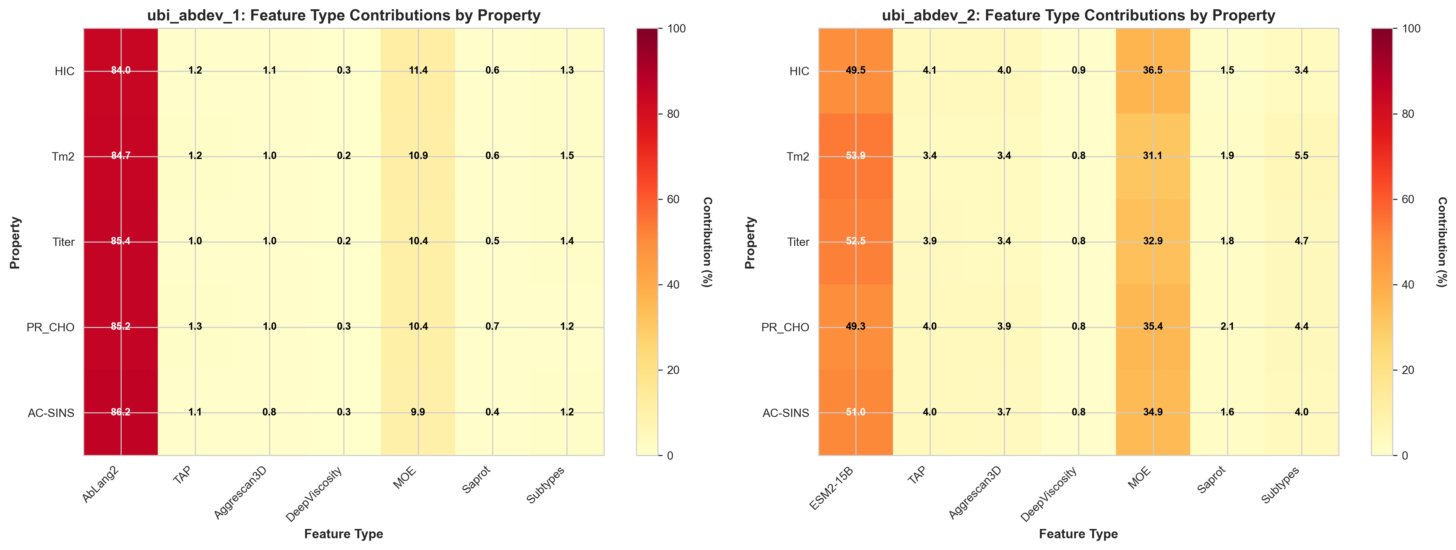
Feature type contributions (%) to predictions for each property in both models
7. The Overfitting Challenge: CV vs Test Performance
One of the most critical findings from the GDPa1 benchmark is the substantial performance degradation from cross-validation to the held-out test set. This reveals a fundamental challenge in antibody developability prediction: models that perform well in CV often fail to generalize to truly unseen antibodies.
7.1 The Performance Gap
Here's a comparison of cross-validation vs. held-out test performance for key models:
| Model | Property | CV ρ | Test ρ | Drop |
|---|---|---|---|---|
| esm2_tap_xgb | Tm2 | 0.328 | 0.102 | -69% |
| esm2_tap_rf | AC-SINS | 0.339 | 0.068 | -80% |
| esm2_tap_xgb | AC-SINS | 0.304 | 0.089 | -71% |
| moe_baseline | HIC | 0.656 | 0.495 | -25% |
| ablang2_elastic_net | HIC | 0.461 | 0.356 | -23% |
| esm2_tap_ridge | HIC | 0.420 | 0.407 | -3% |
Key Observation: Linear Models Generalize Better
Tree-based models (RF, XGBoost) show catastrophic performance drops (69-80% degradation), while linear models (Ridge, ElasticNet) maintain much more consistent performance (3-25% degradation).
This pattern holds across all properties, making linear models with strong regularization the clear choice for antibody developability prediction with limited training data.
7.2 Why Do Complex Models Overfit?
The benchmark provides several insights into why tree-based models struggle:
1. Limited Training Data (246 antibodies)
Tree-based models excel with thousands of training examples. With only 246 antibodies:
- • Decision trees memorize training patterns rather than learning generalizable features
- • Feature interactions learned in CV don't transfer to test antibodies from different sequence spaces
- • Early stopping and max_depth constraints aren't sufficient to prevent overfitting
2. High-Dimensional Feature Space
- • Curse of dimensionality: Tree-based models struggle when features >> samples
- • Spurious correlations: With many features, random correlations appear in training data
- • Linear models benefit: Regularization naturally handles high-dimensional sparse data
3. Distribution Shift Between CV and Test
The held-out test set may have antibodies from different:
- • Sequence families: Different V/J gene usage patterns
- • CDR compositions: Novel amino acid combinations not seen in training
- • Biophysical property ranges: Extreme values that push model extrapolation
Linear models, by learning smooth decision boundaries, handle distribution shifts more gracefully than complex decision trees.
7.3 Fold-Wise Performance Variance
Beyond average CV performance, examining variance across folds reveals how consistently models perform across all 5 biophysical properties. High fold-to-fold variance indicates unstable predictions—a hallmark of overfitting. The hierarchical_cluster_IgG_isotype_stratified_fold strategy creates challenging test sets where models must generalize to antibodies from different sequence clusters. This analysis is critical because real-world developability requires models that perform consistently across diverse antibody designs, not just high average performance on favorable splits.
Comprehensive Fold-Wise Analysis Across All Properties
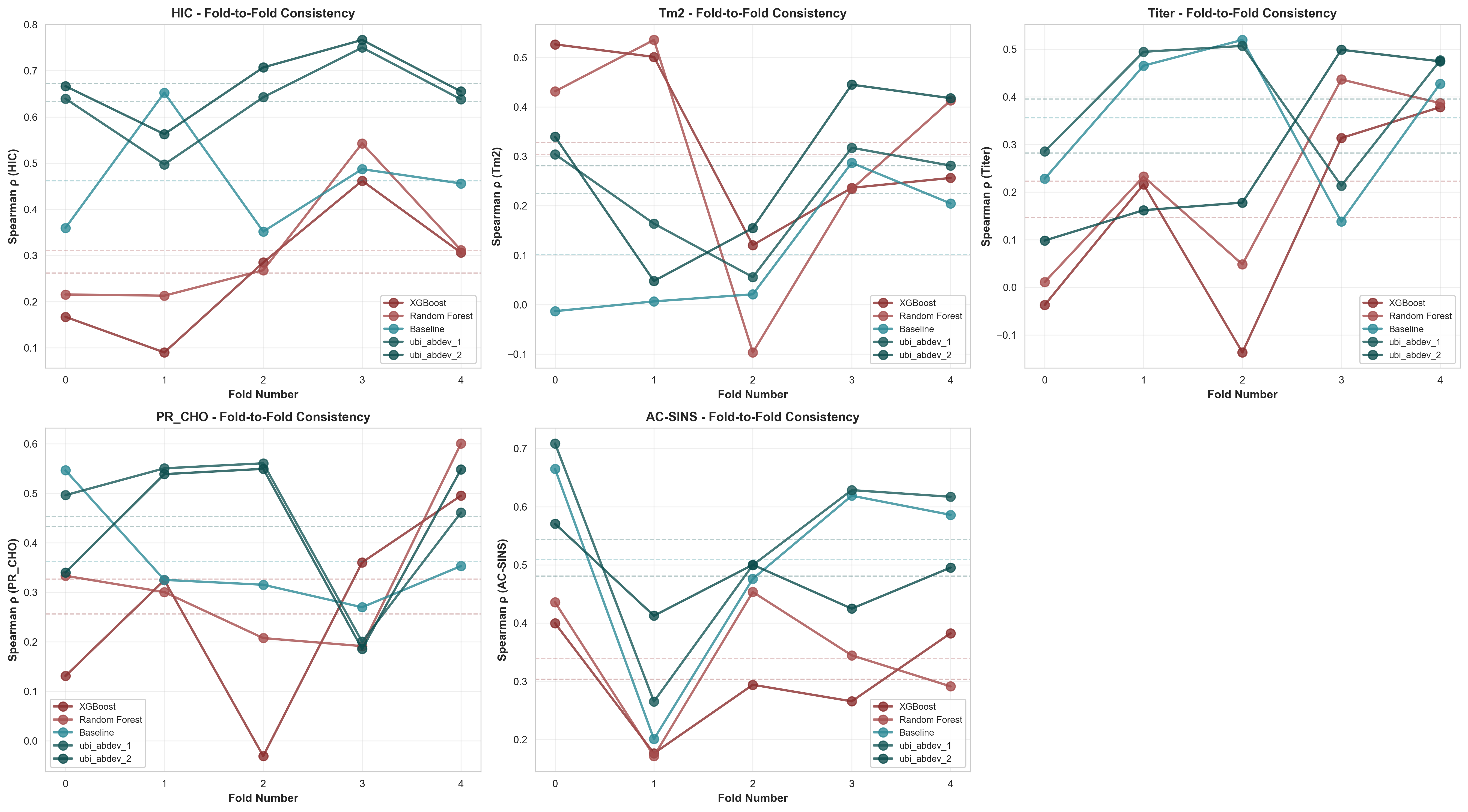
Fold-to-fold performance for all 5 properties. Each panel shows the same 5 models across 5 CV folds (out-of-fold predictions). Dashed horizontal lines indicate model means. Key observations: (1) Tree-based models (red/brown) show extreme fold-to-fold swings indicating overfitting, (2) HIC predictions are most stable across all models, while Tm2 and Titer show the highest variance, reflecting inherent prediction difficulty.
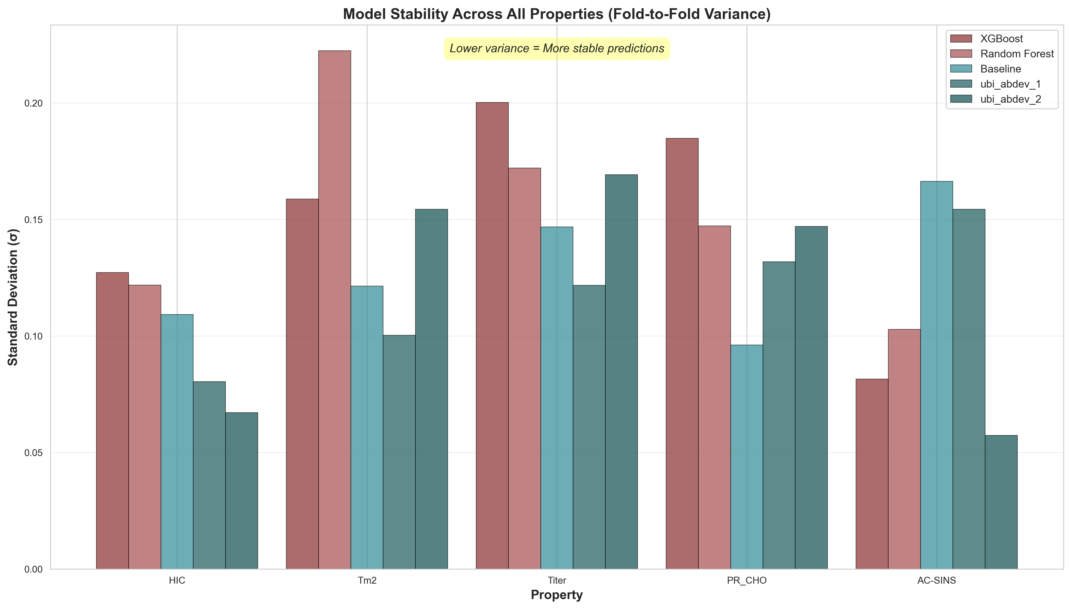
Model stability comparison across all properties. Lower standard deviation (σ) indicates more consistent predictions. Property-specific patterns: HIC and AC-SINS predictions are most stable, while Titer and Tm2 show higher variance across all models—suggesting these properties are inherently harder to predict from sequence features alone.
Property-Specific Performance Patterns
Different properties show distinct variance patterns, revealing which biophysical measurements are more predictable from sequence:
✓ Most Stable Properties
- • HIC (Hydrophobic Interaction Chromatography): All models show relatively low variance (σ < 0.13). UniBio's ubi_abdev_2 achieves σ=0.067 with mean ρ=0.672. Hydrophobicity appears well-captured by language model embeddings.
- • AC-SINS (Self-Association): ubi_abdev_2 shows remarkably low variance (σ=0.057) despite complex aggregation mechanisms. ubi_abdev_1 achieves highest mean (ρ=0.544) but with higher variance (σ=0.154).
⚠ Most Variable Properties
- • Tm2 (Thermal Stability): Highest variance for tree models (RF: σ=0.222, XGBoost: σ=0.159). Even UniBio models show moderate variance (σ=0.100-0.154). Stability depends on complex structural factors beyond sequence.
- • Titer (Expression Level): Second most variable property. XGBoost shows extreme instability (σ=0.200, with negative correlations in some folds). Expression is influenced by cell-line specific factors not captured in sequence.
While we don't yet have held-out test results for our improved models, their strong CV performance combined with the use of regularized linear models suggests they will generalize better than tree-based baselines. The benchmark provides a standardized framework for future evaluation.
8. UbiTools: Making Developability Assessment Accessible
At UniBio Intelligence, we're building UbiTools—an integrated platform that makes antibody developability assessment accessible to researchers and organizations of all sizes. Coming soon, UbiTools will provide:
UbiTools Platform Features
1. Automated Feature Computation
Simply provide antibody sequences (VH/VL), and UbiTools automatically computes:
- Protein language model embeddings (ESM-2, AbLang2)
- TAP physicochemical descriptors
- Structure-based features
2. Multi-Model Inference
Access predictions from multiple models:
- UniBio's improved models: ubi_abdev_1 and ubi_abdev_2
- Best open source models: Top performing models from the abdev-benchmark
- Ensemble predictions: Combine multiple models for robust estimates
Interested in early access? We're looking for pilot partners to help shape the platform. Contact us at contact@unibiointelligence.com to learn more.
Conclusion: Advancing Therapeutic Antibody Development
The GDPa1 benchmark has established a crucial foundation for antibody developability prediction. Our analysis reveals:
- Overfitting is the primary challenge: Complex models fail to generalize from 246 training antibodies
- Linear models with regularization win: ElasticNet and Ridge consistently outperform RF/XGBoost on unseen data
- Feature engineering matters most: Combining multiple feature types (AbLang2 + ESM-2 + TAP) improves predictions more than model complexity
Get Involved
Explore the benchmark and contribute your own models:
- Benchmark Repository: github.com/ginkgobioworks/abdev-benchmark
- Competition: Ginkgo Antibody Developability Competition
- Dataset: GDPa1 on Hugging Face
- Contact Us: contact@unibiointelligence.com
Acknowledgements
This work builds on the foundation laid by the abdev-benchmark repository and the generous contributions of the research community.
Benchmark Contributors
- • Ginkgo Datapoints Team (Lood van Niekerk, Seth Ritter, Joshua Moller)
- • Nels Thorsteinson
- • Nathaniel Blalock, Ameya Kulkarni, and Jeonghyeon Kim (Romero Lab)
- • Shyam C. and Valentin Badea (Harvard DBMI) - for feature engineering and model development
- • Tamarind Bio
- • Netsanet Gebremedhin
- • All contributors to the abdev-benchmark GitHub repository
- • Open-source tool developers whose methods enabled comprehensive feature engineering (see Related Citations below)
- • The broader antibody engineering community for advancing computational methods and sharing datasets
Citation
If you found this analysis helpful or use insights from this work, please cite:
@misc{ubi2025antibodydevelopabilityanalysis,
  author = {UniBio Intelligence},
  title = {Machine Learning for Antibody Developability: Advancing Therapeutic Design with the GDPa1 Benchmark},
  year = {2025},
  url = {https://unibiointelligence.com/blog/antibody-developability-analysis},
  note = {Accessed: 2025-12-22}
}
Related Citations
This work builds on numerous computational methods and datasets. When using these approaches, please cite the original papers:
Dataset & Benchmark
- GDPa1: Mason, D. M., et al. (2024). The antibody developability benchmark. bioRxiv.doi:10.1101/2024.10.10.616558v2
Protein Language Models
- AbLang2: Olsen, T. H., et al. (2024). AbLang2: A universal sequence-based antibody language model. Communications Biology, 7(1), 942.doi:10.1038/s42003-024-06561-3
- ESM-2: Lin, Z., et al. (2023). Evolutionary-scale prediction of atomic-level protein structure with a language model. Science, 379(6637), 1123-1130.doi:10.1126/science.ade2574
Structure Prediction
- ImmuneBuilder: Abanades, B., Wong, W.K., Boyles, F., et al. (2023). ImmuneBuilder: Deep-Learning models for predicting the structures of immune proteins. Communications Biology, 6, 575.doi:10.1038/s42003-023-04927-7
- ABodyBuilder3: Kenlay, H., Dreyer, F.A., Cutting, D., Nissley, D., Deane, C.M. (2024). ABodyBuilder3: improved and scalable antibody structure predictions. Bioinformatics, 40(10), btae576.doi:10.1093/bioinformatics/btae576
- Boltz-2: Wohlwend, J., et al. (2024). Boltz-2: Accurate protein structure prediction at scale. bioRxiv.doi:10.1101/2024.11.19.624167
- AlphaFold 3: Abramson, J., et al. (2024). Accurate structure prediction of biomolecular interactions with AlphaFold 3. Nature, 630, 493–500.doi:10.1038/s41586-024-07487-w
Biophysical Property Prediction
- Aggrescan3D: Kuriata, A., et al. (2019). Aggrescan3D (A3D) 2.0: prediction and engineering of protein solubility. Nucleic Acids Research, 47(W1), W300-W307.doi:10.1093/nar/gkz321
- SaProt: Su, J., et al. (2024). SaProt: Protein Language Modeling with Structure-aware Vocabulary. ICLR 2024.OpenReview
- TAP (Therapeutic Antibody Profiler): Raybould, M. I. J., et al. (2019). Five computational developability guidelines for therapeutic antibody profiling. PNAS, 116(10), 4025-4030.doi:10.1073/pnas.1810576116
Molecular Descriptors
- MOE (Molecular Operating Environment): Chemical Computing Group ULC. Molecular Operating Environment (MOE), 2024.08. Montreal, QC, Canada.chemcomp.com
References
[1]
Jain, T., Sun, T., Durand, S., Hall, A., Houston, N. R., Nett, J. H., ... & Tessier, P. M. (2017). Biophysical properties of the clinical-stage antibody landscape. Proceedings of the National Academy of Sciences, 114(5), 944-949. https://www.pnas.org/doi/10.1073/pnas.1616408114
[2]
Raybould, M. I. J., Marks, C., Krawczyk, K., Taddese, B., Nowak, J., Lewis, A. P., ... & Deane, C. M. (2019). Five computational developability guidelines for therapeutic antibody profiling. Proceedings of the National Academy of Sciences, 116(10), 4025-4030. https://www.pnas.org/doi/10.1073/pnas.1810576116
[3]
Ginkgo Datapoints. (2025). Announcing the Antibody Developability Prediction Competition. Hugging Face Blog. https://huggingface.co/blog/ginkgo-datapoints/2025-abdev-competition
[4]
Bethea, D., Wu, S. J., Luo, J., Hyun, L., Lacy, E. R., Teplyakov, A., ... & Xu, Y. (2012). Mechanisms of self-association of a human monoclonal antibody CNTO607. Protein Engineering, Design and Selection, 25(10), 531-537. https://academic.oup.com/peds/article/25/10/531/1574828
[5]
Lippow, S. M., Wittrup, K. D., & Tidor, B. (2007). Computational design of antibody-affinity improvement beyond in vivo maturation. Nature Biotechnology, 25(10), 1171-1176. https://www.nature.com/articles/nbt1336
[6]
Tiller, K. E., Chowdhury, R., Li, T., Ludwig, S. D., Sen, S., Maranas, C. D., & Tessier, P. M. (2017). Facile affinity maturation of antibody variable domains using natural diversity mutagenesis. Frontiers in Immunology, 8, 986. https://www.frontiersin.org/articles/10.3389/fimmu.2017.00986/full
[7]
Kelly, R. L., Geoghegan, J. C., Feldman, J., Jain, T., Kauke, M., Le, D., ... & Wittrup, K. D. (2021). Polyreactivity and polyspecificity in therapeutic antibody development: risk factors for failure in preclinical and clinical development campaigns. mAbs, 13(1), 1999195. https://www.tandfonline.com/doi/full/10.1080/19420862.2021.1999195
[8]
Lilyestrom, W. G., Yadav, S., Shire, S. J., & Scherer, T. M. (2013). Monoclonal antibody self-association, cluster formation, and rheology at high concentrations. The Journal of Physical Chemistry B, 117(21), 6373-6384. https://pubs.acs.org/doi/10.1021/jp4008152
[9]
Chennamsetty, N., Voynov, V., Kayser, V., Helk, B., & Trout, B. L. (2009). Design of therapeutic proteins with enhanced stability. Proceedings of the National Academy of Sciences, 106(29), 11937-11942. https://www.pnas.org/doi/10.1073/pnas.0904191106
[10]
Mei, S., Wang, Z., Guo, Q., Wang, G., Zhang, Y., Huang, Y., ... & Zeng, J. (2024). A machine learning strategy for the identification of key in silico descriptors and prediction models for IgG monoclonal antibody developability properties. Communications Biology, 7, 891. https://www.nature.com/articles/s42003-024-06561-3
[11]
Lin, Z., Akin, H., Rao, R., Hie, B., Zhu, Z., Lu, W., ... & Rives, A. (2023). Evolutionary-scale prediction of atomic-level protein structure with a language model. Science, 379(6637), 1123-1130. https://www.science.org/doi/10.1126/science.ade2574
[12]
Olsen, T. H., Moal, I. H., & Deane, C. M. (2022). AbLang: an antibody language model for completing antibody sequences. Bioinformatics Advances, 2(1), vbac046. https://academic.oup.com/bioinformaticsadvances/article/2/1/vbac046/6609807
[13]
Shuai, R. W., Ruffolo, J. A., & Gray, J. J. (2022). IgLM: Infilling language modeling for antibody sequence design. Cell Systems, 13(12), 979-989. https://www.cell.com/cell-systems/fulltext/S2405-4712(22)00405-0
[14]
Kuriata, A., Iglesias, V., Kurcinski, M., Ventura, S., & Kmiecik, S. (2019). Aggrescan3D standalone package for structure-based prediction of protein aggregation properties. Bioinformatics, 35(17), 3222-3224. https://academic.oup.com/bioinformatics/article/35/17/3222/5304703
[15]
Yang, Y., Perissinotti, L., Krainak, E., Xu, Y., & Ji, X. (2024). Machine Learning Models for Predicting Monoclonal Antibody Biophysical Properties from Molecular Dynamics Simulations and Deep Learning-Based Surface Descriptors. Molecular Pharmaceutics, 21(10), 5285-5296. https://pubs.acs.org/doi/10.1021/acs.molpharmaceut.4c00804
[16]
Makowski, E. K., Kinnunen, P. C., Huang, J., Wu, L., Smith, M. D., Wang, T., ... & Tessier, P. M. (2022). Co-optimization of therapeutic antibody affinity and specificity using machine learning models that generalize to novel mutational space. Nature Communications, 13, 3788. https://www.nature.com/articles/s41467-022-31457-3
[17]
Akbar, R., Robert, P. A., Pavlović, M., Jeliazkov, J. R., Snapkov, I., Slabodkin, A., ... & Greiff, V. (2022). A compact vocabulary of paratope-epitope interactions enables predictability of antibody-antigen binding. Cell Reports, 34(11), 108856. https://www.cell.com/cell-reports/fulltext/S2211-1247(21)00162-3
[18]
UniBio Intelligence & Ginkgo Bioworks. (2025). abdev-benchmark: Baseline models for antibody developability prediction. GitHub Repository. https://github.com/ginkgobioworks/abdev-benchmark/
[19]
Wang, X., Zhu, Y., Wu, Z., Zhang, Y., & Xu, J. (2025). PROPERMAB: an integrative framework for in silico prediction of antibody developability using machine learning. mAbs, 17(1), 2474521. https://www.tandfonline.com/doi/full/10.1080/19420862.2025.2474521
[20]
Ruffolo, J. A., Chu, L. S., Mahajan, S. P., & Gray, J. J. (2024). Antibody structure prediction using interpretable deep learning. Patterns, 5(2), 100406. https://www.cell.com/patterns/fulltext/S2666-3899(21)00315-5
[21]
Greenman, C., & Mazor, Y. (2021). Machine learning applications in antibody discovery, design and developability. Expert Opinion on Biological Therapy, 21(12), 1613-1622. https://www.tandfonline.com/doi/full/10.1080/14712598.2021.1967338
[22]
Strokach, A., Becerra, D., Corbi-Verge, C., Perez-Riba, A., & Kim, P. M. (2020). Fast and flexible protein design using deep graph neural networks. Cell Systems, 11(4), 402-411. https://www.cell.com/cell-systems/fulltext/S2405-4712(20)30299-0
[23]
Watson, J. L., Juergens, D., Bennett, N. R., Trippe, B. L., Yim, J., Eisenach, H. E., ... & Baker, D. (2023). De novo design of protein structure and function with RFdiffusion. Nature, 620(7976), 1089-1100. https://www.nature.com/articles/s41586-023-06415-8
[24]
Hie, B. L., Shanker, V. R., Xu, D., Bruun, T. U. J., Weidenbacher, P. A., Tang, S., ... & Kim, P. S. (2024). Efficient evolution of human antibodies from general protein language models. Nature Biotechnology, 42(2), 275-283. https://www.nature.com/articles/s41587-023-01763-2
[25]
Fernández-Quintero, M. L., Kroell, K. B., Bacher, L. M., Loeffler, J. R., Quoika, P. K., Georges, G., ... & Liedl, K. R. (2024). Molecular surface descriptors to predict antibody developability: sensitivity to parameters, structure models, and conformational sampling. mAbs, 16(1), 2362788. https://www.tandfonline.com/doi/full/10.1080/19420862.2024.2362788
Related Content
Explore more from UniBio Intelligence: